Visualizing Neural Network Compression

Abstract: Often, the best models are the biggest. Too big for you or me to run. Luckily, with model compression we can drastically reduce the size of these models. This article runs through a simple way to compress neural network weights with k-means quantization. Through interactive visuals, I'll explore a simple approach as well as it's shortcomings (error).

Introduction

Modern deep learning is quite extraordinary. I don't need to convince you. You've likely seen the latest generative art models.

From

These models generate detailed and stunning outputs. And yet, they are just transforming input data over and over again until a desirable output. For example, large models like

Size enables amazing capabilities, but also limits who can run the models. Most people don't have fast GPUs with lots of memory. To fit these models on our hardware, we must to reduce the size.

Sharing as Compression

In this article I'll use the weight sharing scheme from

Suppose you owned 20 dogs. An army of golden retrievers. And also suppose you are on the market for dog toys.

Should you buy 20 toys for all 20 dogs? That would be quite expensive! If each toy was $20, then you'd pay $400. (as you can tell I love the number 20)

But you are a clever one you. You could reason that buying 5 toys would be totally fine. The dogs can share. Now your bill would only be $100 for the 5 toys.

Not only that, but sharing might increase the amount of fun the dogs have! But sharing might also favor the more dominant and strong dogs. There is a tradeoff, but we're on a budget, so it's fine.

Morale of the short story: sharing under constraints is reasonable. More than that. It's a good idea. Don't pay for more than you need to if you're on a budget. But also don't delude yourself in thinking there aren't downsides because there are.

In some sense we are compressing our budget through sharing.

Sharing Pixels

Images and neural network weights are held in similar data structures so let's first look at the more intuitive image use-case. It will be the same.

For image compression, the goal is to reduce the memory footprint while maintaining what the original image looked like. In other words, the budget is the size.

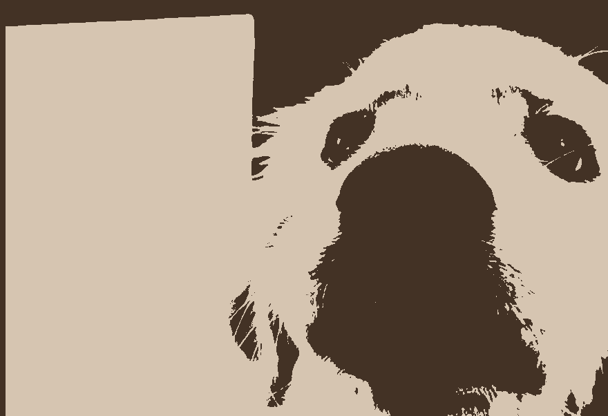
As you know, images are made up of tons of small colored squares: pixels. I'll start with a 880 pixels wide by 602 pixels tall image of this cutest golden retriever you've ever seen.

In total, there are 4,824,160 colors in the image ($880 \cdot 602$): one for each pixel. Each color is represented by three numbers: red, green, and blue that mix together to make that color. In total this one image is storing nearly 15 million numbers! That is quite a bit!

Instead of each pixel having it's own unique color, why not pick the most important colors and force the pixels to share? Exactly like the previous example with buying toys. Instead of storing three numbers per every pixel, I can now just store a few colors that each pixel can index into.

First, I'll take an average over all the pixels to get the one most important color. Making all the pixels share that one pixel I get:

Compressed

1 color

Original

4,824,160 colors

It is significantly smaller in terms of memory, but looks nothing like the dog.

Now, let's share two colors instead of just one.

Compressed

2 colors

Original

4,824,160 colors

Starting to look like a dog!

So what happens when we increase beyond two colors? Let's try!

Compressed

2 colors

Original

4,824,160 colors

After sharing just 256 colors, the images look remarkably similar. And we're only storing just 256 colors instead of nearly 5 million!

Instead of storing three numbers per pixel, I store one that indexes into the shared important color pixels.

Above, the window shows a small portion of the pixels at eight (or three bit since $2^3$) color compression. As you can see, each pixel is a single three bit number that indexes into the shared colors which contains three numbers each. Hover over the image to move the mini window!

Quantifying Error

You get the point. We can indeed reduce our budget without losing the main use-case.

You can apply this exact method to the weight matrix in a linear layer of a neural network! But in some ways, the problem is harder.

First, how do we know when we've compressed the weights adequately? With the image example, we could just view all the different quantizations and see which was closest. How would you do this for arbitrary numbers learned in a neural network? You can't just look at them and see if they look good.

Instead, we need a metric that tells us how good the compression is compared to the original.

Let's go back to the image case because it's more intuitive. I will assume that the image compression when the colors are far away from the true colors. In other words, the difference between the original pixels and the compressed pixels is how bad our error is.

As you can see, when the images look very similar, the red error is almost nonexistent. I can further summarize the error with an average into one number.

This example shows it's entirely possible to attach a number to how good the compression is.

Matrix Multiplication

Then, how do we attach a number to the compression error for neural networks? Again, we aren't viewing them as images. So what makes their compression good or not?

Take this three layer neural network $$\text{ReLU}\left(\text{ReLU}\left(xW_1^T + b_1\right)W_2^T + b_2\right)W_3^T + b_3.\tag{2}$$ where $W_i$ are weights and $b_i$ are biases at layer $i$.

Just like image example, we must create a metric based on the use-case. Since almost all the operations on the weights are matrix multiplies, it might be a good idea to take this operation into account as the use-case. In other words, how does the approximate compressed weights differ after a matrix multiplication of the same input compared to the original/exact weights? It might be the case the the multiplies and adds amplify or even hide element-wise error!

With matrix multiplication we are doing a linear combination of the columns of the matrix defined by each number in the input vector. Namely, $Wx = y$ where $W$ is the matrix, $x$ is the column vector, and $y$ is the output of the matrix multiply. Alternatively, think of $W$ as transforming $x$ into $y$.

I can also define $W$ compressed/quantized as $Q$. The $Q$ matrix transforms the input $x$ into some approximate output $\hat{y}$. Since $Q$ is an approximate $W$, the output would also be approximate. I can then express the differences between the outputs $y$ and $\hat{y}$ in a single error term $$\begin{align*}\text{error} &:= \frac{||y - \hat{y}||}{||y||}\tag{3}\end{align*}$$ which is the size of how wrong the approximation is after the matrix multiply.

And since $Wx = y$ and $Qx = \hat{y}$ I can write the equation $(3)$ only in terms of the inputs as

$$\begin{align*} \frac{||y - \hat{y}||}{||y||} = \frac{||Wx - Qx||}{||Wx||}\tag{4}\\ \end{align*}$$

simply by how I defined things. Nothing new yet.

As is turns out, I can factor the error term in $(4)$ into one term that only contains $W$ and other term that contains both $Q$ and $W$ through the steps $$\begin{align*} \frac{||Wx - Qx||}{||Wx||} &= \frac{||(W-Q)x||}{||Wx||}\\ &= \frac{||(W-Q)W^{-1}y||}{||Wx||}&&\text{since } x = W^{-1}y\\ &\leq \frac{||W-Q|| \ ||W^{-1}|| \ ||y||}{||Wx||}&&\text{since } ||AB|| \leq ||A|| \ ||B||\\ &= \frac{||W-Q|| \ ||W^{-1}|| \ ||Wx||}{||Wx||}&&\text{since } ||Wx|| = ||y||\\ &= ||W-Q|| \ ||W^{-1}||\\ &= \frac{||W||}{||W||} \ ||W-Q|| \ ||W^{-1}||\\ &= \left(||W|| \ ||W^{-1}||\right) \left(\frac{||W-Q||}{||W||}\right). \tag{5}\\ \end{align*}$$ where the norm applied to a matrix is the matrix operator norm induced by the 1-norm.

The first term $W$ as $||W|| \ ||W^{-1}||$ is a very useful number in many applications for linear problems: the condition number. The second term $\frac{||W-Q||}{||W||}$ looks quite similar to the image pixel error case. What's really important is that there is error inherent to the original matrix in the condition number. The condition number then scales the difference between original and compressed (the second term).

Let's see what error looks like on some different weight matrices!

Unsurprisingly, the error drops drastically when we have enough weights to share. Additionally, the error gets close to zero and the quantization makes the weights 4 times smaller! That is a total win!

My second observation is that not all weight distributions have the same condition number. Additionally, it seems to be that k-means quantization does quite well, if not better, when the condition number is higher. How could this be? Surely this is wrong.

Yes I'm partially wrong. The condition number, which scales the error term, becomes very high with spiked values (outliers). This makes sense given small errors to these values would change the matrix multiply drastically. But at the very same time, k-means is known to be sensitive to outliers (to a fault). So k-means gives an entire shared weight to the outlier. Most of the time this is terrible for compression, but since k-means quantization is non-linear, it's a total win for this small example.

This is a bit of a tangent, but k-means has a clear advantage over linear quantization schemes in terms of minimizing error depending on how large your weight matrix is.

More layers

Okay, but what about more than just one weight matrix.

Instead of just one layer of weights, now I'll scale up to multiple layers with a real usable model.

I'll use a simple autoencoder architecture takes takes images of handwritten digits¹ (0 through 9) and attempts to reconstruct the image after a bottleneck.

In

import torch
model = torch.nn.Sequential(
    torch.nn.Linear(28*28, 1000),
    torch.nn.ReLU(),
    torch.nn.Linear(1000, 256),
    torch.nn.ReLU(),
    torch.nn.Linear(256, 256),
    torch.nn.ReLU(),
    torch.nn.Linear(256, 1000),
    torch.nn.ReLU(),
    torch.nn.Linear(1000, 28*28),
    torch.nn.Sigmoid()
)

import torch
model = torch.nn.Sequential(
    torch.nn.Linear(28*28, 1000),
    torch.nn.ReLU(),
    torch.nn.Linear(1000, 256),
    torch.nn.ReLU(),
    torch.nn.Linear(256, 256),
    torch.nn.ReLU(),
    torch.nn.Linear(256, 1000),
    torch.nn.ReLU(),
    torch.nn.Linear(1000, 28*28),
    torch.nn.Sigmoid()
)

The training and definitions are in

I quantized the model's weights and biases. Then, I loaded the PyTorch weights directly in my own

As you can see, with a small number of bits, the output reconstruction is terrible. But as you pass some threshold it becomes quite good and doesn't improve by too much. Very importantly, the quantized models are four times smaller than the original.

To get a condition number and some semblance of error prediction, I iterated over each layer and took the max condition number. As shown below and in

import torch
def matrix_operator_norm1(A):
    """||A||"""
    return torch.linalg.matrix_norm(A, 1)
def cond1(A):
    """||A||||A^{-1}||"""
    A_inverse = torch.linalg.pinv(A)
    return matrix_operator_norm1(A)*matrix_operator_norm1(A_inverse)
@torch.no_grad()
def combined_cond(model): 
    """max i ( ||W_i|||||W_i^{-1}|| )"""
    weights = [param for name, param in model.named_parameters() if "weight" in name]
    cond_nums = [cond1(param).item() for param in weights]
    return max(cond_nums)
print(combined_cond(model)) # 54168.84375

import torch
def matrix_operator_norm1(A):
    """||A||"""
    return torch.linalg.matrix_norm(A, 1)
def cond1(A):
    """||A||||A^{-1}||"""
    A_inverse = torch.linalg.pinv(A)
    return matrix_operator_norm1(A)*matrix_operator_norm1(A_inverse)
@torch.no_grad()
def combined_cond(model): 
    """max i ( ||W_i|||||W_i^{-1}|| )"""
    weights = [param for name, param in model.named_parameters() if "weight" in name]
    cond_nums = [cond1(param).item() for param in weights]
    return max(cond_nums)
print(combined_cond(model)) # 54168.84375

Despite this neural network having a high maximum condition number of 54,168, the outputs look quite good after k-means quantization: the reconstruction is accurate.

I speculate again that with extra shared numbers to spare, k-means was sensitive to the outlier which caused the high condition number, thereby masking the large effects and driving down the entire error term from equation $(5)$.

Conclusion

Perhaps not a satisfying ending, but here we are. Overall, yes it's possible to quantize the vast majority of weights in your neural network with little error. But make sure you're using the right error metrics!

Also make sure to take into account how the weights are used so you know exactly how much you can compress. It may be that taking into account non-linearities and other architectures could further develop the operator norm and relative error into something very useful for neural networks.

Acknowledgments

• I thank myself
  Donny Bertucci
  for writing the article and
  Adam Perer
  for discussing ideas and for valuable feedback
• My interest in model compression came from conversations with
  Venkat Sivaraman
• Inspiration to use k-means came from watching this
  video
  (which evidently is by the author of that Deep Compression Paper)
• Observable Plot
  was extremely useful
• SveltePress
  is really awesome out of the box
• KaTeX
  for math equations

Cite

@misc{bertucci2023viscompress,
   author = {Bertucci, Donald and Perer, Adam},
   title  = {{Visualizing Neural Network Compression}},
   year   = {2023}
}

@misc{bertucci2023viscompress,
   author = {Bertucci, Donald and Perer, Adam},
   title  = {{Visualizing Neural Network Compression}},
   year   = {2023}
}